Learning Outcomes
- Display data graphically and translate graphs: stemplots, histograms, and box plots.
- Recognize, depict, and calculate the measures of location of data: quartiles and percentiles.
For most of the work yous practise in this book, yous volition utilise a histogram to display the data. One advantage of a histogram is that it can readily display big information sets. A dominion of thumb is to use a histogram when the data set consists of [latex]100[/latex] values or more.
Ahistogram consists of face-to-face (bordering) boxes. Information technology has both a horizontal axis and a vertical axis. The horizontal axis is labeled with what the data represents (for instance, altitude from your home to school). The vertical axis is labeled either frequency or relative frequency (or percent frequency or probability). The graph will have the same shape with either label. The histogram (like the stemplot) can give you the shape of the data, the center, and the spread of the information.
The relative frequency is equal to the frequency for an observed value of the data divided by the total number of data values in the sample. (Remember, frequency is defined as the number of times an respond occurs.) If:
- [latex]f[/latex] = frequency
- [latex]northward[/latex] = total number of data values (or the sum of the private frequencies), and
- [latex]RF[/latex] = relative frequency,
then [latex]\displaystyle{R}{F}=\frac{{f}}{{n}}[/latex]
For example, if three students in Mr. Ahab's English form of [latex]40[/latex] students received from [latex]90[/latex]% to [latex]100[/latex]%, then, [latex]\displaystyle{f}={3},{due north}={twoscore}[/latex], and [latex]{R}{F}=\frac{{f}}{{n}}=\frac{{3}}{{40}}={0.075}[/latex]. [latex]vii.five[/latex]% of the students received [latex]90–100[/latex]%. [latex]90–100[/latex]% are quantitative measures.
To construct a histogram, first decide how many bars or intervals, also chosen classes, represent the data. Many histograms consist of five to [latex]15[/latex] bars or classes for clarity. The number of bars needs to exist chosen. Choose a starting point for the starting time interval to exist less than the smallest data value. A user-friendly starting point is a lower value carried out to one more than decimal identify than the value with the about decimal places. For example, if the value with the most decimal places is [latex]6.one[/latex] and this is the smallest value, a convenient starting bespeak is [latex]6.05[/latex] ([latex]6.ane – 0.05 = 6.05[/latex]). We say that [latex]half dozen.05[/latex] has more precision. If the value with the almost decimal places is [latex]2.23[/latex] and the lowest value is [latex]1.five[/latex], a convenient starting point is [latex]1.495[/latex] ([latex]1.5 – 0.005 = ane.495[/latex]). If the value with the nigh decimal places is [latex]iii.234[/latex] and the everyman value is [latex]1.0[/latex], a convenient starting signal is [latex]0.9995[/latex] ([latex]1.0 – 0.0005 = 0.9995[/latex]). If all the data happen to be integers and the smallest value is two, then a convenient starting point is [latex]one.5[/latex] ([latex]two – 0.5 = 1.five[/latex]). Also, when the starting point and other boundaries are carried to 1 boosted decimal place, no information value will fall on a purlieus. The side by side 2 examples go into detail about how to construct a histogram using continuous data and how to create a histogram using discrete information.
Spotter the following video for an case of how to describe a histogram.
Case
The post-obit data are the heights (in inches to the nearest one-half inch) of [latex]100[/latex] male semiprofessional soccer players. The heights are continuous data, since height is measured.
[latex]60[/latex]; [latex]60.5[/latex]; [latex]61[/latex]; [latex]61[/latex]; [latex]61.5[/latex]
[latex]63.5[/latex]; [latex]63.5[/latex]; [latex]63.five[/latex]
[latex]64[/latex]; [latex]64[/latex]; [latex]64[/latex]; [latex]64[/latex]; [latex]64[/latex]; [latex]64[/latex]; [latex]64[/latex]; [latex]64.5[/latex]; [latex]64.v[/latex]; [latex]64.five[/latex]; [latex]64.five[/latex]; [latex]64.5[/latex]; [latex]64.five[/latex]; [latex]64.5[/latex]; [latex]64.566[/latex]; [latex]66[/latex]; [latex]66[/latex]; [latex]66[/latex]; [latex]66[/latex]; [latex]66[/latex]; [latex]66[/latex]; [latex]66[/latex]; [latex]66[/latex]; [latex]66[/latex]; [latex]66.5[/latex]; [latex]66.5[/latex]; [latex]66.5[/latex]; [latex]66.five[/latex]; [latex]66.five[/latex]; [latex]66.5[/latex]; [latex]66.five[/latex]; [latex]66.v[/latex]; [latex]66.5[/latex]; [latex]66.5[/latex]; [latex]66.five[/latex]; [latex]67[/latex]; [latex]67[/latex]; [latex]67[/latex]; [latex]67[/latex]; [latex]67[/latex]; [latex]67[/latex]; [latex]67[/latex]; [latex]67[/latex]; [latex]67[/latex]; [latex]67[/latex]; [latex]67[/latex]; [latex]67[/latex]; [latex]67.5[/latex]; [latex]67.5[/latex]; [latex]67.v[/latex]; [latex]67.5[/latex]; [latex]67.5[/latex]; [latex]67.5[/latex]; [latex]67.5[/latex]
[latex]68[/latex]; [latex]68[/latex]; [latex]69[/latex]; [latex]69[/latex]; [latex]69[/latex]; [latex]69[/latex]; [latex]69[/latex]; [latex]69[/latex]; [latex]69[/latex]; [latex]69[/latex]; [latex]69[/latex]; [latex]69[/latex]; [latex]69.five[/latex]; [latex]69.5[/latex]; [latex]69.five[/latex]; [latex]69.v[/latex]; [latex]69.5[/latex]
[latex]70[/latex]; [latex]70[/latex]; [latex]70[/latex]; [latex]70[/latex]; [latex]70[/latex]; [latex]70[/latex]; [latex]70.5[/latex]; [latex]seventy.five[/latex]; [latex]70.5[/latex]; [latex]71[/latex]; [latex]71[/latex]; [latex]71[/latex]
[latex]72[/latex]; [latex]72[/latex]; [latex]72[/latex]; [latex]72.5[/latex]; [latex]72.five[/latex]; [latex]73[/latex]; [latex]73.5[/latex]; [latex]74[/latex]
The smallest information value is [latex]60[/latex]. Since the data with the most decimal places has ane decimal (for instance, [latex]61.5[/latex]), nosotros want our starting point to have 2 decimal places. Since the numbers [latex]0.five[/latex], [latex]0.05[/latex], [latex]0.005[/latex], etc. are convenient numbers, apply [latex]0.05[/latex] and decrease it from [latex]threescore[/latex], the smallest value, for the convenient starting point.
[latex]60 – 0.05 = 59.95[/latex] which is more precise than, say, [latex]61.v[/latex] past one decimal place. The starting signal is, then, [latex]59.95[/latex].
The largest value is [latex]74[/latex], then [latex]74 + 0.05 = 74.05[/latex] is the ending value.
Next, calculate the width of each bar or class interval. To calculate this width, subtract the starting signal from the ending value and separate past the number of confined (you must choose the number of bars you want). Suppose you cull eight confined.
Annotation
Nosotros volition round up to two and brand each bar or course interval 2 units wide. Rounding up to two is one manner to prevent a value from falling on a boundary. Rounding to the next number is often necessary even if it goes against the standard rules of rounding. For this example, using [latex]i.76[/latex] as the width would also work. A guideline that is followed by some for the width of a bar or class interval is to have the square root of the number of data values and then circular to the nearest whole number, if necessary. For case, if in that location are [latex]150[/latex] values of data, take the square root of [latex]150[/latex] and round to [latex]12[/latex] bars or intervals.
The boundaries are:
- [latex]59.95[/latex]
- [latex]59.95 + ii = 61.95[/latex]
- [latex]61.95 + two = 63.95[/latex]
- [latex]63.95 + 2 = 65.95[/latex]
- [latex]65.95 + 2 = 67.95[/latex]
- [latex]67.95 + 2 = 69.95[/latex]
- [latex]69.95 + 2 = 71.95[/latex]
- [latex]71.95 + two = 73.95[/latex]
- [latex]73.95 + two = 75.95[/latex]
The heights [latex]60[/latex] through [latex]61.5[/latex] inches are in the interval [latex]59.95–61.95[/latex]. The heights that are [latex]63.5[/latex] are in the interval [latex]61.95–63.95[/latex]. The heights that are [latex]64[/latex] through [latex]64.5[/latex] are in the interval [latex]63.95–65.95[/latex]. The heights [latex]66[/latex] through [latex]67.five[/latex] are in the interval [latex]65.95–67.95[/latex]. The heights [latex]68[/latex] through [latex]69.5[/latex] are in the interval [latex]67.95–69.95[/latex]. The heights [latex]70[/latex] through [latex]71[/latex] are in the interval [latex]69.95–71.95[/latex]. The heights [latex]72[/latex] through [latex]73.five[/latex] are in the interval [latex]71.95–73.95[/latex]. The height [latex]74[/latex] is in the interval [latex]73.95–75.95[/latex].
The following histogram displays the heights on the [latex]10[/latex]-axis and relative frequency on the [latex]y[/latex]-axis.

Try It
The following information are the shoe sizes of [latex]50[/latex] male students. The sizes are continuous data since shoe size is measured. Construct a histogram and summate the width of each bar or form interval. Suppose yous choose six bars.
[latex]ix[/latex]; [latex]9[/latex]; [latex]ix.5[/latex]; [latex]ix.5[/latex]; [latex]x[/latex]; [latex]10[/latex]; [latex]ten[/latex]; [latex]10[/latex]; [latex]10[/latex]; [latex]10[/latex]; [latex]10.5[/latex]; [latex]10.5[/latex]; [latex]x.5[/latex]; [latex]10.5[/latex]; [latex]10.v[/latex]; [latex]x.v[/latex]; [latex]x.five[/latex]; [latex]10.v[/latex]
[latex]eleven[/latex]; [latex]11[/latex]; [latex]11[/latex]; [latex]11[/latex]; [latex]xi[/latex]; [latex]11[/latex]; [latex]11[/latex]; [latex]11[/latex]; [latex]11[/latex]; [latex]xi[/latex]; [latex]11[/latex]; [latex]11[/latex]; [latex]xi[/latex]; [latex]11.v[/latex]; [latex]xi.five[/latex]; [latex]11.five[/latex]; [latex]11.v[/latex]; [latex]11.5[/latex]; [latex]eleven.5[/latex]; [latex]xi.v[/latex]
[latex]12[/latex]; [latex]12[/latex]; [latex]12[/latex]; [latex]12[/latex]; [latex]12[/latex]; [latex]12[/latex]; [latex]12[/latex]; [latex]12.5[/latex]; [latex]12.v[/latex]; [latex]12.5[/latex]; [latex]12.five[/latex]; [latex]14[/latex]
Example
The following data are the number of books bought past fifty office-fourth dimension college students at ABC Higher. The number of books is discrete data, since books are counted.
[latex]1[/latex]; [latex]1[/latex]; [latex]1[/latex]; [latex]ane[/latex]; [latex]ane[/latex]; [latex]1[/latex]; [latex]1[/latex]; [latex]1[/latex]; [latex]1[/latex]; [latex]1[/latex]; [latex]1[/latex]
[latex]2[/latex]; [latex]2[/latex]; [latex]2[/latex]; [latex]2[/latex]; [latex]2[/latex]; [latex]2[/latex]; [latex]2[/latex]; [latex]2[/latex]; [latex]2[/latex]; [latex]2[/latex]
[latex]3[/latex]; [latex]iii[/latex]; [latex]3[/latex]; [latex]3[/latex]; [latex]3[/latex]; [latex]3[/latex]; [latex]3[/latex]; [latex]3[/latex]; [latex]iii[/latex]; [latex]iii[/latex]; [latex]3[/latex]; [latex]iii[/latex]; [latex]3[/latex]; [latex]3[/latex]; [latex]3[/latex]; [latex]3[/latex]
[latex]4[/latex]; [latex]four[/latex]; [latex]4[/latex]; [latex]4[/latex]; [latex]four[/latex]; [latex]4[/latex]
[latex]five[/latex]; [latex]v[/latex]; [latex]5[/latex]; [latex]v[/latex]; [latex]five[/latex]
[latex]6[/latex]; [latex]6[/latex]
Xi students buy i book. 10 students buy ii books. Xvi students buy three books. Six students purchase 4 books. Five students buy v books. 2 students buy six books.
Because the data are integers, subtract [latex]0.5[/latex] from [latex]1[/latex], the smallest data value and add together [latex]0.5[/latex] to [latex]6[/latex], the largest data value. Then the starting signal is [latex]0.five[/latex] and the ending value is [latex]vi.5[/latex].
Next, summate the width of each bar or class interval. If the data are discrete and there are not too many different values, a width that places the data values in the middle of the bar or grade interval is the most user-friendly. Since the data consist of the numbers [latex]i[/latex], [latex]ii[/latex], [latex]iii[/latex], [latex]4[/latex], [latex]5[/latex], [latex]6[/latex], and the starting indicate is [latex]0.5[/latex], a width of one places the [latex]1[/latex] in the middle of the interval from [latex]0.five[/latex] to [latex]1.5[/latex], the [latex]2[/latex] in the middle of the interval from [latex]one.5[/latex] to [latex]2.five[/latex], the [latex]iii[/latex] in the middle of the interval from [latex]two.5[/latex] to [latex]3.5[/latex], the [latex]4[/latex] in the eye of the interval from _______ to _______, the [latex]5[/latex] in the middle of the interval from _______ to _______, and the _______ in the middle of the interval from _______ to _______ .
Summate the number of bars as follows:
where [latex]1[/latex] is the width of a bar. Therefore, bars = [latex]six[/latex].
The following histogram displays the number of books on the [latex]x[/latex]-centrality and the frequency on the [latex]y[/latex]-centrality.

USING THE TI-83, 83+, 84, 84+ Computer
Create the histogram for Example ii.
- Printing Y=. Press CLEAR to delete any equations.
- Press STAT 1:EDIT. If L1 has information in it, pointer up into the name L1, press CLEAR and and then arrow down. If necessary, do the same for L2.
- Into L1, enter [latex]ane[/latex], [latex]2[/latex], [latex]3[/latex], [latex]4[/latex], [latex]v[/latex], [latex]half dozen[/latex].
- Into L2, enter [latex]xi[/latex], [latex]10[/latex], [latex]16[/latex], [latex]six[/latex], [latex]5[/latex], [latex]2[/latex].
- Printing WINDOW. Set up Xmin = [latex].5[/latex], Xscl = [latex](half dozen.5 – .v)/six[/latex], Ymin = [latex]–ane[/latex], Ymax = [latex]xx[/latex], Yscl = [latex]1[/latex], Xres = [latex]ane[/latex].
- Press 2nd Y=. Starting time past pressing 4:Plotsoff ENTER.
- Press 2nd Y=. Printing 1:Plot1. Press ENTER. Pointer down to Type. Pointer to the tertiary picture show (histogram). Printing ENTER.
- Arrow down to Xlist: Enter L1 (2d one). Arrow down to Freq. Enter L2 (2nd 2).
- Printing GRAPH.
- Use the TRACE primal and the arrow keys to examine the histogram.
Try It
The following data are the number of sports played by l student athletes. The number of sports is discrete data since sports are counted.
[latex]1[/latex]; [latex]one[/latex]; [latex]one[/latex]; [latex]1[/latex]; [latex]1[/latex]; [latex]ane[/latex]; [latex]1[/latex]; [latex]1[/latex]; [latex]1[/latex]; [latex]1[/latex]; [latex]1[/latex]; [latex]1[/latex]; [latex]1[/latex]; [latex]1[/latex]; [latex]1[/latex]; [latex]1[/latex]; [latex]i[/latex]; [latex]one[/latex]; [latex]1[/latex]; [latex]1[/latex]
[latex]ii[/latex]; [latex]two[/latex]; [latex]2[/latex]; [latex]2[/latex]; [latex]2[/latex]; [latex]two[/latex]; [latex]ii[/latex]; [latex]two[/latex]; [latex]ii[/latex]; [latex]2[/latex]; [latex]2[/latex]; [latex]2[/latex]; [latex]2[/latex]; [latex]2[/latex]; [latex]2[/latex]; [latex]ii[/latex]; [latex]2[/latex]; [latex]2[/latex]; [latex]2[/latex]; [latex]two[/latex]; [latex]2[/latex]; [latex]two[/latex]
[latex]three[/latex]; [latex]3[/latex]; [latex]iii[/latex]; [latex]iii[/latex]; [latex]3[/latex]; [latex]3[/latex]; [latex]three[/latex]; [latex]three[/latex]
[latex]twenty[/latex] student athletes play one sport. [latex]22[/latex] student athletes play ii sports. 8 student athletes play three sports.
Fill in the blanks for the post-obit sentence. Since the data consist of the numbers [latex]1[/latex], [latex]2[/latex], [latex]3[/latex], and the starting point is [latex]0.v[/latex], a width of i places the [latex]ane[/latex] in the middle of the interval [latex]0.5[/latex] to _____, the [latex]2[/latex] in the middle of the interval from _____ to _____, and the [latex]3[/latex] in the center of the interval from _____ to _____.
Case
Using this data ready, construct a histogram.
| Number of Hours My Classmates Spent Playing Video Games on Weekends | ||||
|---|---|---|---|---|
| [latex]9.95[/latex] | [latex]x[/latex] | [latex]2.25[/latex] | [latex]xvi.75[/latex] | [latex]0[/latex] |
| [latex]19.5[/latex] | [latex]22.v[/latex] | [latex]7.5[/latex] | [latex]xv[/latex] | [latex]12.75[/latex] |
| [latex]5.five[/latex] | [latex]11[/latex] | [latex]10[/latex] | [latex]20.75[/latex] | [latex]17.5[/latex] |
| [latex]23[/latex] | [latex]21.9[/latex] | [latex]24[/latex] | [latex]23.75[/latex] | [latex]18[/latex] |
| [latex]twenty[/latex] | [latex]fifteen[/latex] | [latex]22.9[/latex] | [latex]eighteen.8[/latex] | [latex]20.5[/latex] |
Try It
The post-obit data represent the number of employees at various restaurants in New York City. Using this data, create a histogram.
[latex]22[/latex]; [latex]35[/latex]; [latex]xv[/latex]; [latex]26[/latex]; [latex]forty[/latex]; [latex]28[/latex]; [latex]18[/latex]; [latex]xx[/latex]; [latex]25[/latex]; [latex]34[/latex]; [latex]39[/latex]; [latex]42[/latex]; [latex]24[/latex]; [latex]22[/latex]; [latex]xix[/latex]; [latex]27[/latex]; [latex]22[/latex]; [latex]34[/latex]; [latex]40[/latex]; [latex]20[/latex]; [latex]38[/latex]; and [latex]28[/latex]
Use [latex]10–xix[/latex] every bit the kickoff interval.
COLLABORATIVE Do
Count the coin (bills and alter) in your pocket or handbag. Your instructor volition record the amounts. As a class, construct a histogram displaying the information. Discuss how many intervals you think is advisable. Y'all may want to experiment with the number of intervals.
Frequency Polygons
Frequency polygons are analogous to line graphs, and but as line graphs make continuous data visually like shooting fish in a barrel to interpret, so too exercise frequency polygons.
To construct a frequency polygon, first examine the data and decide on the number of intervals, or class intervals, to use on the [latex]ten[/latex]-centrality and [latex]y[/latex]-axis. Subsequently choosing the appropriate ranges, begin plotting the data points. After all the points are plotted, draw line segments to connect them.
example
A frequency polygon was constructed from the frequency table below.
| Frequency Distribution for Calculus Final Examination Scores | |||
|---|---|---|---|
| Lower Jump | Upper Bound | Frequency | Cumulative Frequency |
| [latex]49.5[/latex] | [latex]59.5[/latex] | [latex]5[/latex] | [latex]five[/latex] |
| [latex]59.5[/latex] | [latex]69.5[/latex] | [latex]10[/latex] | [latex]15[/latex] |
| [latex]69.five[/latex] | [latex]79.v[/latex] | [latex]thirty[/latex] | [latex]45[/latex] |
| [latex]79.five[/latex] | [latex]89.5[/latex] | [latex]forty[/latex] | [latex]85[/latex] |
| [latex]89.5[/latex] | [latex]99.v[/latex] | [latex]15[/latex] | [latex]100[/latex] |
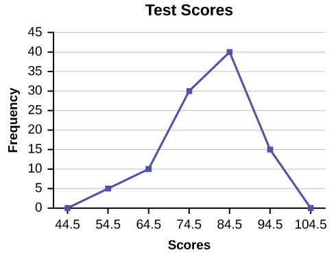
The outset label on the [latex]ten[/latex]-axis is [latex]44.5[/latex]. This represents an interval extending from [latex]39.5[/latex] to [latex]49.v[/latex]. Since the lowest test score is [latex]54.5[/latex], this interval is used only to let the graph to affect the [latex]x[/latex]-axis. The point labeled [latex]54.5[/latex] represents the next interval, or the get-go "real" interval from the tabular array, and contains v scores. This reasoning is followed for each of the remaining intervals with the indicate [latex]104.five[/latex] representing the interval from [latex]99.v[/latex] to [latex]109.5[/latex]. Once more, this interval contains no information and is simply used so that the graph will touch the [latex]x[/latex]-centrality. Looking at the graph, we say that this distribution is skewed because 1 side of the graph does not mirror the other side.
Try Information technology
Construct a frequency polygon of U.S. Presidents' ages at inauguration shown in the tabular array.
| Age at Inauguration | Frequency |
|---|---|
| [latex]41.5–46.5[/latex] | [latex]iv[/latex] |
| [latex]46.5–51.5[/latex] | [latex]eleven[/latex] |
| [latex]51.five–56.v[/latex] | [latex]14[/latex] |
| [latex]56.five–61.5[/latex] | [latex]9[/latex] |
| [latex]61.5–66.5[/latex] | [latex]iv[/latex] |
| [latex]66.5–71.5[/latex] | [latex]ii[/latex] |
Frequency polygons are useful for comparing distributions. This is accomplished by overlaying the frequency polygons drawn for unlike data sets.


